Amazon Quick Follow Up - Market Analysis

In previous article I couldn’t hold myself other than roasting Amazon Quick user experience. To be fair, these criticism is still on constructive intentions and I’m sure that Amazon Quick team are already making their utmost effort to resolve all the problems. In this article, we will be more optimistic and practical.

Now - Amazon Quick is powerful. It has a major potential, and I have no doubt that it will improve further in the near future. With that being said, I will continue to Hamza’s work on the use case of the tool.

AirBnb Market Analysis: Berlin vs. Munich

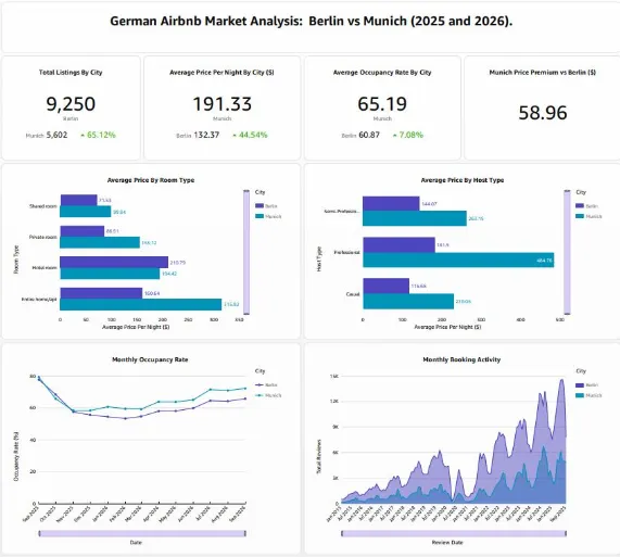
Following steps are to create a quicksight dashboard that provides insight on AirBnb market - comparing Berlin to Munich. Once ready, we will be able to review some important numbers per city: such as occupancy rate or total number of listings. We will also have a bar chart to compare price average by room type or a line chart to review booking activities per month. The dashboard covers 2025 to 2026 data however it can also continuously feed data and can be used for the upcoming years. A dashboard as this one can be useful for businesses offering services to AirBnb owners or to policy makers researching on the topic. Following steps will take place in order to create the dashboard:

1. We are going to first fetch the reference dataset.
2. We will perform transformation steps to make data analytics-ready (gold layer).
3. We will load the data inside Databricks.
4. We will visualize the data with Quicksight.

Pre-requisites

While following the guide below, you will need to use Databricks, python, uv package manager, dbt libraries in Python and finally access to Amazon Quick and Quicksight. If you feel uncomfortable about signing up for any of these, feel free to not follow up the rest of the article (and please let me know if you have any alternative approaches in mind).

Step by Step Quicksight Dashboard Creation

1. Pull the data from the reference source. Search “Munich” and “Berlin” in the page and make sure you download Listings, Calendar and Reviews for both cities.

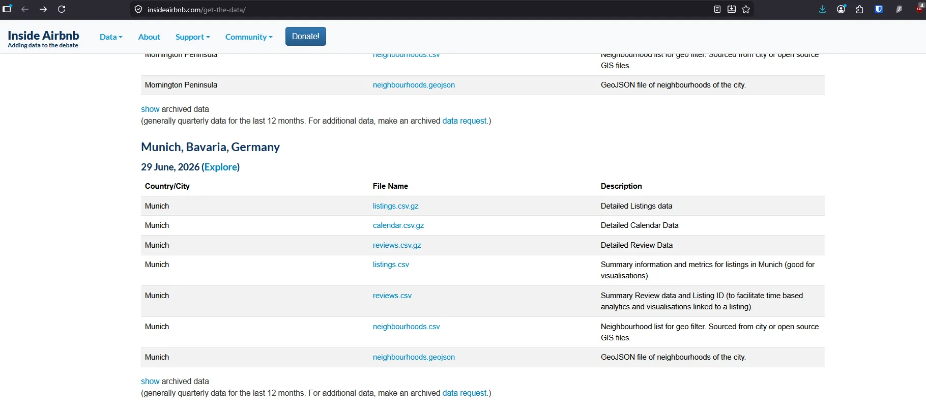
2. Navigate to Databricks sign-up page and create an account for free. I know, it’s annoying to go through all the process, but at least it’s free (and a tip: you can use a temporary account).

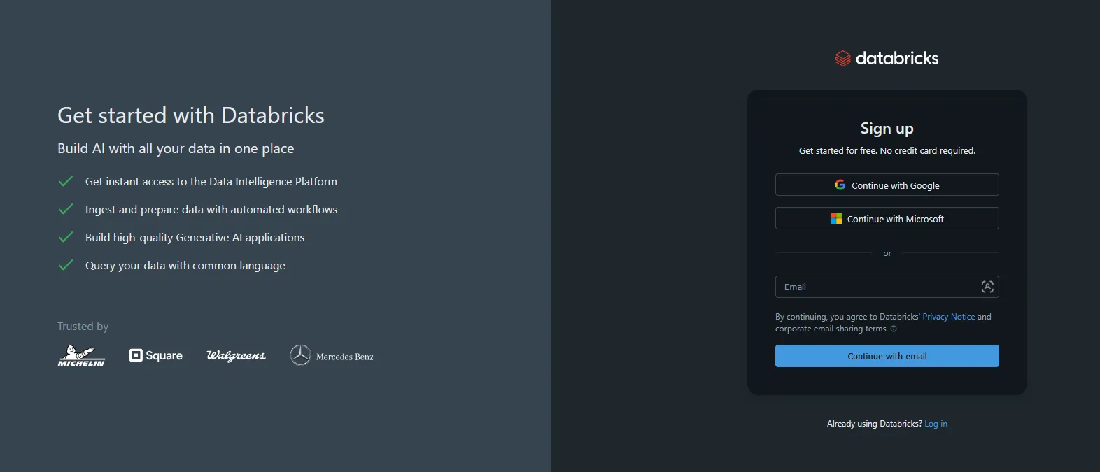
3. At Databricks main page find Catalog -> Schema -> Create Table and finally upload all CSV files downloaded.
4. Open your favorite IDE (e.g. VS Code, Kiro, Cursor etc.) and create a new project folder. Following, run pip install uv to activate uv.
5. By using uv (a powerful package manager in python) we run the following commands one by one:

uv init     # initializes uv and generates core files
uv sync     # creates the virtual environment for isolation 
uv add dbt-core             # adds dbt-core for dbt functionality
uv add dbt-databricks       # adds databricks specific library of dbt
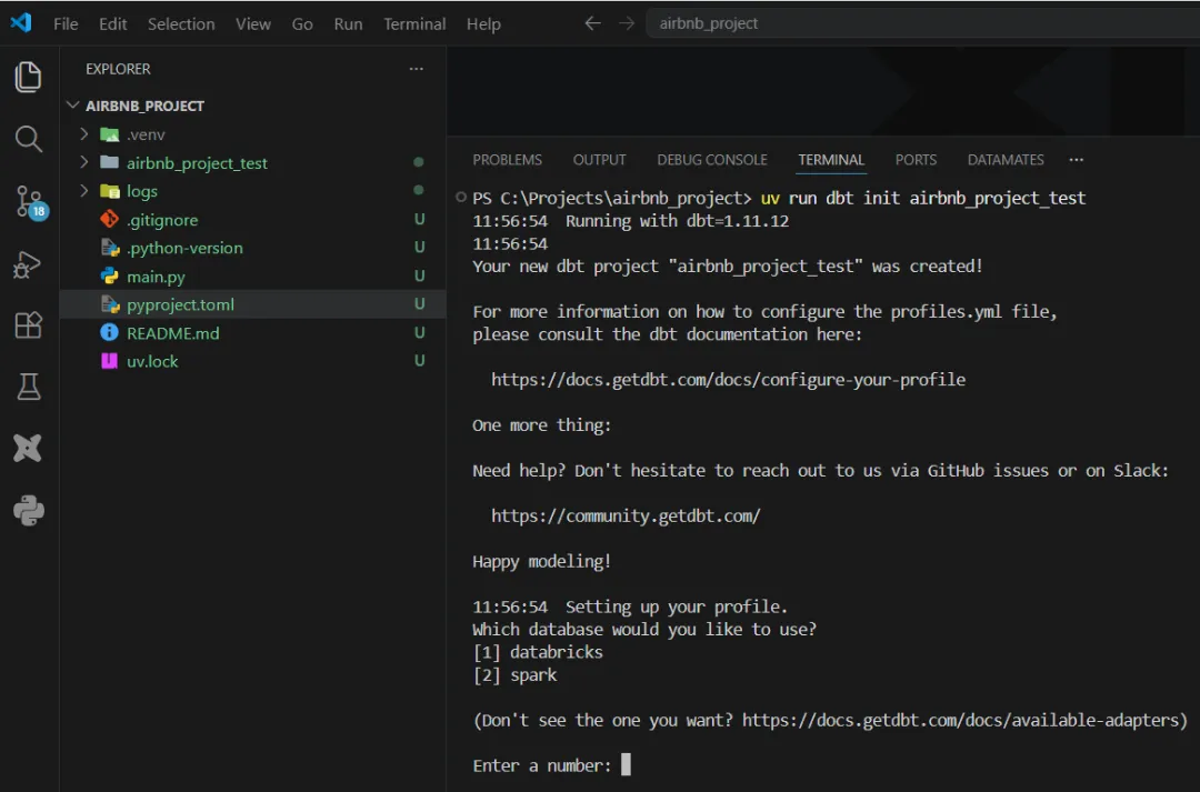
uv run dbt init airbnb_project      # starts airbnb_project as a project

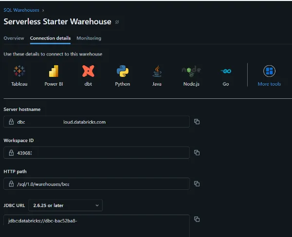
6. Once you run the final command: uv run dbt init airbnb_project, this will request several details to connect to your databricks data. In order to fill, find all the relevant data in your Databricks dashboard:

• Compute -> Serverless Starter Warehouse -> Connection Details
• Save server hostname and http path
• Click create personal access token at the right top of the screen
• Provide all details back to Databricks connection.
• Dbt will create a profiles.yml file from this location: ~/.dbt/profiles.yml - paste this file into your project folder.

7. Test your connection between dbt and Databricks by running in terminal: dbt debug - if all checks pass, we’re good to go.

Pit-stop: What is dbt and what did we build so far?

dbt is used for data transformation. It cleans out raw, bronze data into silver and eventually to analysis-ready gold form. All of the magic of data transformation happens inside dbt. To explain dbt in simple terms, it is the Transormation in the ELT (Extract, Load, Transform) process. It doesn’t store the data, it simply takes the data from the data warehouse, then performs transformation steps using SQL. Eventually it populates the transformed data.

Until this part, we initialized our project, installed all dbt required python libraries and secured a connection between our remote Databricks database and our local python codebase. Next step is to transform the data by using some simple SQL queries.

Implementation of Medallion Architecture

As mentioned earlier, a medallion architecture of data is used, to make the raw data analysis ready. Once the data is imported, the project should have a models folder as shared below:

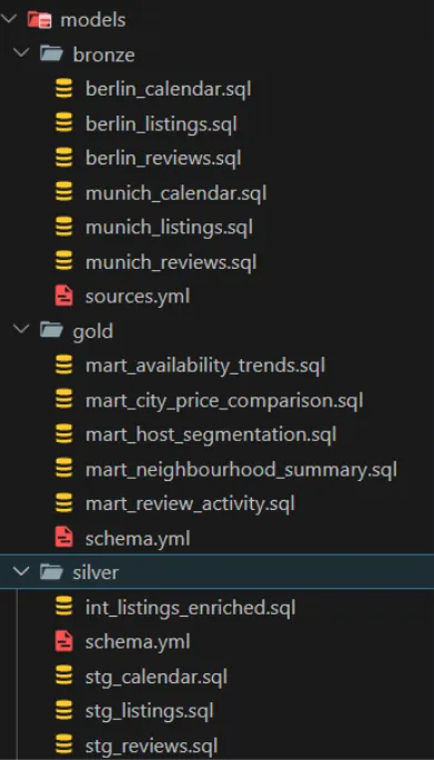
This means that inside of Databricks warehouse, three schemas will be populated: bronze, silver and gold in the format of tables.

8. Create sources.yml inside bronze folder and add the following declaration:

version: 2

sources:
  - name: berlin
    catalog: airbnb
    schema: berlin
    tables:
      - name: listings_raw
      - name: reviews_raw
      - name: calendar_raw

  - name: munich
    catalog: airbnb
    schema: munich
    tables:
      - name: listings_raw
      - name: reviews_raw
      - name: calendar_raw

9. Fill in the rest of the SQL files, same as in the reference repository. If you’re stuck with any part, please get in touch and we will help you.

10. Once added, implement dbt on each medallion by running the commands in order:

uv run dbt run --select bronze
uv run dbt run --select silver
uv run dbt run --select gold

And take a good look on the output. Each run is providing some insight on the implementation.

Pit-stop: What is implemented in medallion architecture?

For each field, the description of queries are explained below:

A. Bronze Layer:

We write simple SQL queries to get the raw data as-is inside the layer. The queries don’t make any changes in the data, simply pulls them.

B. Silver Layer:

Four models are built in this layer:

• Stg_listings:
  • Unioned Berlin and Munich raw tables from bronze layer
  • Cleaned up the price column. The price column had $ signs, ‘,’dates and Booleans mixed together.
  • Casted all columns to correct types
  • Filtered out rows where price was 0 for an Airbnb property
• Stg_calendar:
  • Unioned Berlin and Munich raw tables from bronze layer
  • Filtered out rows where date was NULL
• Stg_reviews:
  • Unioned Berlin and Munich raw tables from bronze layer
  • Filtered out rows where date was NULL
• Int_listings_enriched:
  • Enrichment on top of the stg_listings model applied. Extra columns for segmentation added, based on different scenarios.

C. Gold Layer:

This is where the analytical steps come into the game. Some important marts are developed for analytical purposes.

• Mart_availability_trends:
  • Tells in which months is the property most occupied.
  • Insight: From September to February, the occupancy percentage in Berlin drops to 25% compared to the other months
• Mart_city_price_comparison:
  • Compare the two cities based on their average price and max price.
  • Insight: Munich costs almost double than Berlin across every room type
• Mart_host_segmentation:
  • Tells about the hosts in the two cities, their reviews and total listings for them
  • Insight: Professional hosts in Munich charge €485 where casual hosts charge €230
• Mart_review_activity:
  • Tells about the review activity in the two cities in different months
  • Insight: Both cities hit had the highes reviews in 2024, with a steep decline in 2020 due to COVID

Connecting Project to Amazon Quicksight & Preparing Metrics and Dashboards

Finally the dataset is ready! And it’s time to connect the DB into Amazon Quick and prepare some data visualisation. We will connect to Amazon Quick, then create a new project, connect the Databricks DB and will start building insights.

1. In the AWS Console, go to search bar and type “QuickSight”.
2. Create a QuickSight Account and then log in.
3. Find the Quick homepage, look for Quicksight -> click Data.
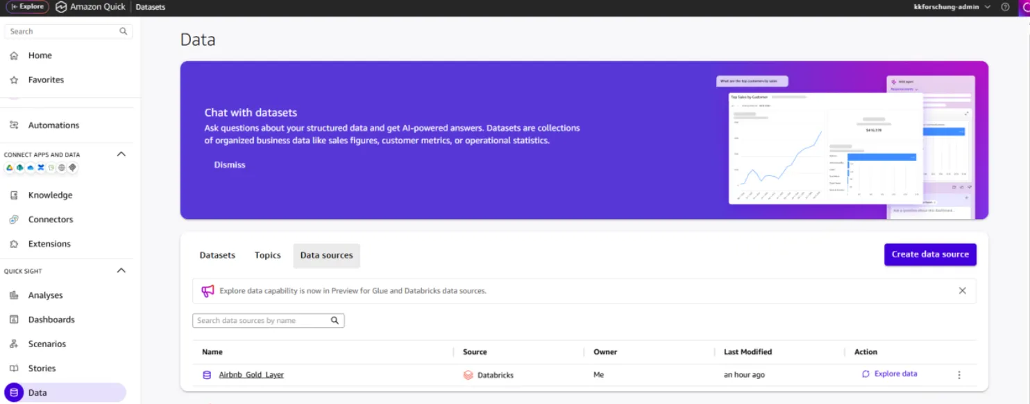
4. You should see a screen similar to below. Click on Data Sources and Click Create Data Source. Following, data sources to connect will be available.

5. Select Databricks as the source and fill in the field similar to values used also when connecting to Databricks:

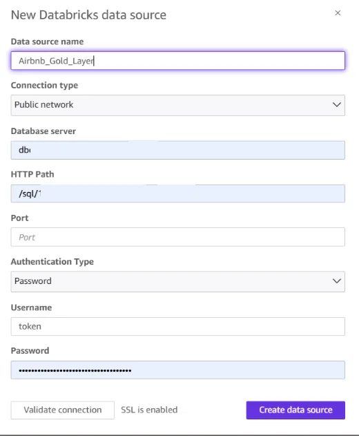
Any data source name can be chosen here. Password is the personal access token which can be generated from Databricks in the top right of the section.

6. After dataset is visible, head on to Analyses section and click Create analysis button. Select any of the dataset and the clear dashboard will be available. At this level, there are three palletes open: Data, Visuals and Sheet. In the Data section, one table is selected and its columns are visible. Visuals section allows user to select a metric type to build. Sheet part is the representation of what is built.

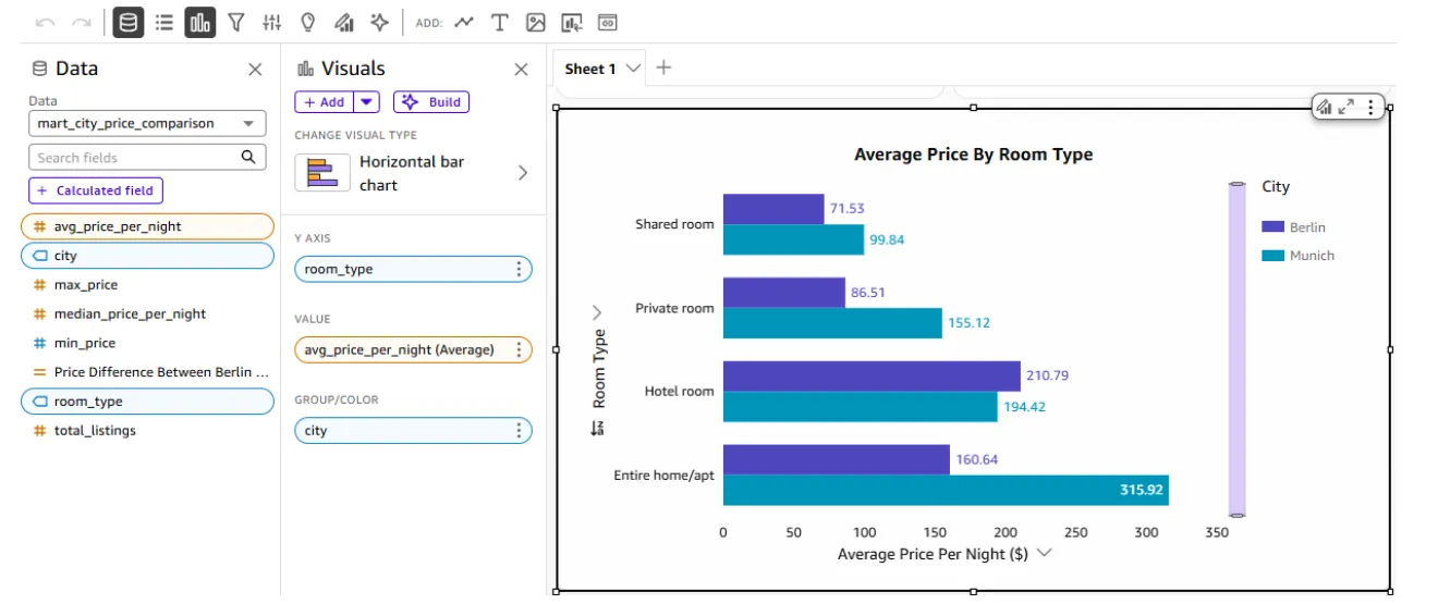
7. The final part is the fun part - creation of the dashboard. To leave some room for the challenge, I don’t provide the full instructions there. Please go ahead and try to build the dashboard yourself. Alternatively try building different type of metrics with the existing data. Anything you believe is worth providing the insight. This is where the real business intelligence kicks into the game.

Final Words on Amazon Quick, Databricks and dbt.

This has been a long article with many details, but we learned a lot of things. We learned how to create a python project for data engineering. We learned how to integrate dbt with use of a uv, an amazing package manager. Not only we uploaded data and connected our Databricks at local level, but we also connected it into Amazon Quick. Finally we created metrics and deployed our first dashboard in Amazon Quick.

These are still beginner steps, lots more can be done and should be done. But this is a great start and is worth experimenting for anyone working with data. If you have further suggestions on the tool, you are welcome to reach out and let’s discuss further!

Until then, enjoy building with Amazon Quick and enjoy working with data.